Soft Diffusion Score Matching for General Corruptions
Super Short Description
- Paper Link
- This paper aims to establish a principled way of training a diffusion model for removing arbitrary linear corruptions which can be modelled by a matrix multiplication with the input. There are overall three contributions: 1. Soft score matching: a novel training objective. They show its relationship with the DSM (Denoising score matching) objective. 2. Momemtum sampler: More detailed image generation along with increased diversity is achieved. 3. Scheduling: They quantify shift in distribution on adding degradation and thereby provide a principled way of deciding how much overall degradation should be at each step.
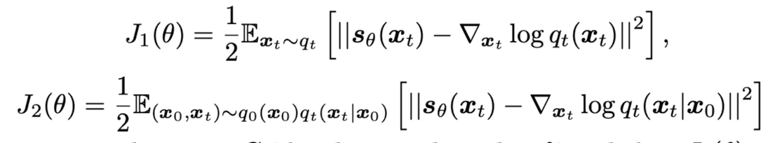
Soft score matching
The authors work with linear corruptions which could be modelled by a matrix multiplication as denoted by C_t below (blur).  {: .align-center}
Uncleared Doubt
The do a network reparametrization making use of the given linear corruption matrix. Instead of moving the network prediction s_{\theta}(x|t) closer to (C_t* x_0 - x_t)/\sigma^2_t, they instead predict h_{\theta}, which is related to s_{\theta} as shown below.  {: .align-center}
Hence, now, C_t*h_{\theta}(x|t) now is trained to be close to C_t * x_0. While it is clear that it is a reparametrization and that the knowledge about the degradation is used, it is not clear what is the advantage of this reparametrization. An ablation study on this would have been helpful.
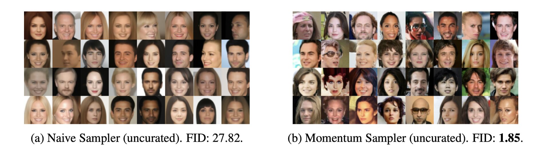
Momentum Sampler
They look at their formulation as a Stochastic differential equation (SDE) and they argue that their SDE formulation is reversible. They discretize the reverse diffusion process to obtain an expression for \Delta x, which when added to x_t, moves it closer to x_0. The expression for \Delta x is shown below.
It is worth noting that there are three expressions above. The first one is doing deblurring (Notice the difference is being taken between the degradation matrices) and the second one is doing denoising. One could also see below the qualitative effect of the momentum sampler.
Scheduling
The authors note that if one degradation step is too large, the network may not be able to learn the score. The quantify the step size by the distance between the two adjacent distributions. They pick the number of intermediate degradation distributions such that the distance between the two adjacent distributions is upper bounded by a given threshold. This threshold denotes the maximum shift in distribution that the network can handle.